
Classifying Cats and Dogs using CNN
Introduction
In this blog post, we will make a Image Classification model using CNN, convolutional neural networks, to tell cats apart from dogs. We will be using the Tensorflow library for model construction and training
import os
from tensorflow import keras
import tensorflow as tf
from tensorflow.keras import utils
Data Import
# location of data
_URL = 'https://storage.googleapis.com/mledu-datasets/cats_and_dogs_filtered.zip'

# download the data and extract it
path_to_zip = utils.get_file('cats_and_dogs.zip', origin=_URL, extract=True)

# construct paths
PATH = os.path.join(os.path.dirname(path_to_zip), 'cats_and_dogs_filtered')

train_dir = os.path.join(PATH, 'train')
validation_dir = os.path.join(PATH, 'validation')

# parameters for datasets
BATCH_SIZE = 32
IMG_SIZE = (160, 160)

# construct train and validation datasets
train_dataset = utils.image_dataset_from_directory(train_dir,
                                                   shuffle=True,
                                                   batch_size=BATCH_SIZE,
                                                   image_size=IMG_SIZE)

validation_dataset = utils.image_dataset_from_directory(validation_dir,
                                                        shuffle=True,
                                                        batch_size=BATCH_SIZE,
                                                        image_size=IMG_SIZE)

# construct the test dataset by taking every 5th observation out of the validation dataset
val_batches = tf.data.experimental.cardinality(validation_dataset)
test_dataset = validation_dataset.take(val_batches // 5)
validation_dataset = validation_dataset.skip(val_batches // 5)
Downloading data from https://storage.googleapis.com/mledu-datasets/cats_and_dogs_filtered.zip
68608000/68606236 [==============================] - 1s 0us/step
68616192/68606236 [==============================] - 1s 0us/step
Found 2000 files belonging to 2 classes.
Found 1000 files belonging to 2 classes.
Let’s take a look at one training dataset.
#retrieves one dataset
train_dataset.take(1)
<TakeDataset element_spec=(TensorSpec(shape=(None, 160, 160, 3), dtype=tf.float32, name=None), TensorSpec(shape=(None,), dtype=tf.int32, name=None))>
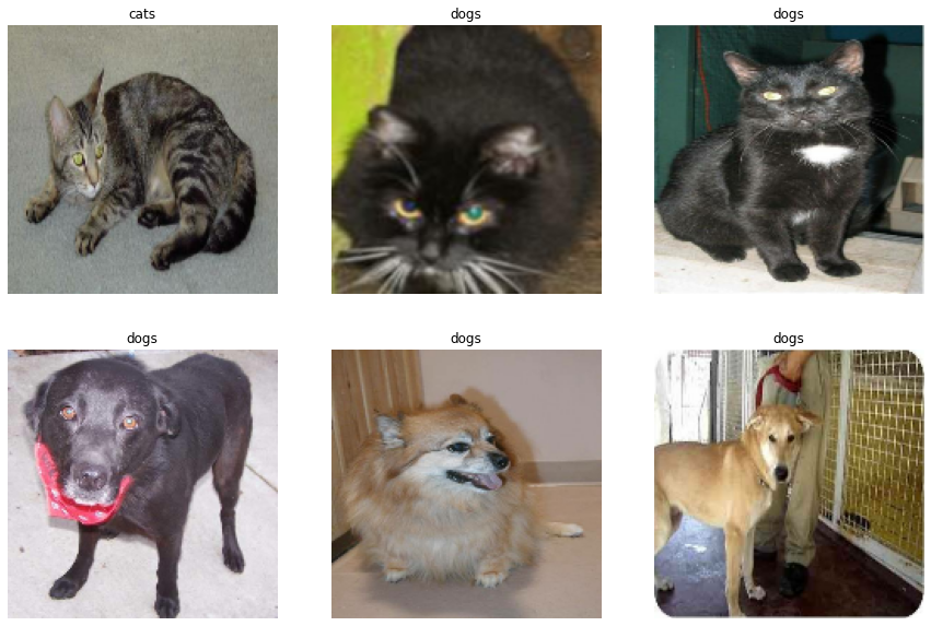
Now, let’s look at our cat and dog images for training.
import matplotlib.pyplot as plt

class_names = train_dataset.class_names

#plots the images from our dataset
plt.figure(figsize=(15, 10))
for images, labels in train_dataset.take(1):
  cat = images[labels==0]
  dog = images[labels==1]
  for i in range(6):
      ax = plt.subplot(2, 3, i + 1)
      if i <=2:
        plt.imshow(cat[i].numpy().astype("uint8"))
        plt.title(class_names[labels[i]])
        plt.axis("off")
      else:
        plt.imshow(dog[i].numpy().astype("uint8"))
        plt.title(class_names[labels[i]])
        plt.axis("off")
We will apply the autotone module to improve performance when reading our data.
AUTOTUNE = tf.data.AUTOTUNE

train_dataset = train_dataset.prefetch(buffer_size=AUTOTUNE)
validation_dataset = validation_dataset.prefetch(buffer_size=AUTOTUNE)
test_dataset = test_dataset.prefetch(buffer_size=AUTOTUNE)
The most basic machine learning model will simply guess the most frequent occurance. To compute the baseline accuracy, let’s take a look at our
#makes a numpy iterator object
labels_iterator= train_dataset.unbatch().map(lambda image, label: label).as_numpy_iterator()
dog_count, cat_count = 0, 0

#counts the cats and dogs in our dataset
for l in labels_iterator:
  if l == 0:
    cat_count += 1
  elif l == 1:
    dog_count += 1

(cat_count, dog_count)
(1000, 1000)
The dog/cat ratio is exactly 50/50, which makes the baseline model as good as a blind guess. We will have to do much better than that!
First Model
To construct our first model, we will be using the Keras module, specifically the sequential model. We will take advantage of the Conv2D layer for data convultion, the MaxPooling layer for dimension reduction, the Dropout layer for reducing overfitting.
from tensorflow.keras import layers

#model using the Sequential function
model1 = keras.Sequential([
    layers.Conv2D(32, (3, 3), activation='relu', input_shape=(160, 160, 3)),
    layers.MaxPooling2D((2, 2)),
    layers.Conv2D(32, (3, 3), activation='relu'),
    layers.MaxPooling2D((2, 2)),
    layers.Flatten(),
    layers.Dropout(0.2),
    layers.Dense(2)
])
Let’s take a look at our model summary.
model1.summary()
Model: "sequential"
_________________________________________________________________
 Layer (type)                Output Shape              Param #
=================================================================
 conv2d (Conv2D)             (None, 158, 158, 32)      896

 max_pooling2d (MaxPooling2D  (None, 79, 79, 32)       0
 )

 conv2d_1 (Conv2D)           (None, 77, 77, 32)        9248

 max_pooling2d_1 (MaxPooling  (None, 38, 38, 32)       0
 2D)

 flatten (Flatten)           (None, 46208)             0

 dropout (Dropout)           (None, 46208)             0

 dense (Dense)               (None, 2)                 92418

=================================================================
Total params: 102,562
Trainable params: 102,562
Non-trainable params: 0
_________________________________________________________________
#compile our model
model1.compile(optimizer='adam',
              loss = tf.keras.losses.SparseCategoricalCrossentropy(from_logits=True),
              metrics = ['accuracy'])

#train our model
history = model1.fit(train_dataset,
                   epochs=20, # how many rounds of training to do
                   validation_data = validation_dataset
)
Epoch 1/20
63/63 [==============================] - 6s 81ms/step - loss: 0.2666 - accuracy: 0.8945 - val_loss: 3.2294 - val_accuracy: 0.5210
Epoch 2/20
63/63 [==============================] - 5s 80ms/step - loss: 0.2454 - accuracy: 0.8995 - val_loss: 3.4499 - val_accuracy: 0.5025
Epoch 3/20
63/63 [==============================] - 5s 80ms/step - loss: 0.1857 - accuracy: 0.9235 - val_loss: 5.4450 - val_accuracy: 0.5186
Epoch 4/20
63/63 [==============================] - 5s 76ms/step - loss: 0.2075 - accuracy: 0.9280 - val_loss: 5.1521 - val_accuracy: 0.5520
Epoch 5/20
63/63 [==============================] - 5s 78ms/step - loss: 0.1928 - accuracy: 0.9295 - val_loss: 5.1780 - val_accuracy: 0.5186
Epoch 6/20
63/63 [==============================] - 5s 76ms/step - loss: 0.3211 - accuracy: 0.9035 - val_loss: 3.7341 - val_accuracy: 0.5347
Epoch 7/20
63/63 [==============================] - 5s 80ms/step - loss: 0.2199 - accuracy: 0.9110 - val_loss: 4.2797 - val_accuracy: 0.5557
Epoch 8/20
63/63 [==============================] - 5s 80ms/step - loss: 0.1482 - accuracy: 0.9375 - val_loss: 5.1100 - val_accuracy: 0.5297
Epoch 9/20
63/63 [==============================] - 5s 78ms/step - loss: 0.1737 - accuracy: 0.9350 - val_loss: 4.5498 - val_accuracy: 0.5681
Epoch 10/20
63/63 [==============================] - 7s 99ms/step - loss: 0.1716 - accuracy: 0.9455 - val_loss: 5.0508 - val_accuracy: 0.5681
Epoch 11/20
63/63 [==============================] - 5s 80ms/step - loss: 0.1859 - accuracy: 0.9315 - val_loss: 4.8768 - val_accuracy: 0.5681
Epoch 12/20
63/63 [==============================] - 5s 81ms/step - loss: 0.1913 - accuracy: 0.9295 - val_loss: 4.0360 - val_accuracy: 0.5248
Epoch 13/20
63/63 [==============================] - 6s 85ms/step - loss: 0.2225 - accuracy: 0.9120 - val_loss: 5.3036 - val_accuracy: 0.5569
Epoch 14/20
63/63 [==============================] - 5s 80ms/step - loss: 0.1480 - accuracy: 0.9420 - val_loss: 5.5931 - val_accuracy: 0.5483
Epoch 15/20
63/63 [==============================] - 5s 80ms/step - loss: 0.1420 - accuracy: 0.9380 - val_loss: 5.9564 - val_accuracy: 0.5631
Epoch 16/20
63/63 [==============================] - 5s 79ms/step - loss: 0.1559 - accuracy: 0.9485 - val_loss: 5.3253 - val_accuracy: 0.5458
Epoch 17/20
63/63 [==============================] - 5s 81ms/step - loss: 0.1264 - accuracy: 0.9540 - val_loss: 6.5667 - val_accuracy: 0.5470
Epoch 18/20
63/63 [==============================] - 5s 78ms/step - loss: 0.1355 - accuracy: 0.9485 - val_loss: 6.2064 - val_accuracy: 0.5173
Epoch 19/20
63/63 [==============================] - 5s 76ms/step - loss: 0.1386 - accuracy: 0.9525 - val_loss: 5.1241 - val_accuracy: 0.5248
Epoch 20/20
63/63 [==============================] - 6s 83ms/step - loss: 0.2408 - accuracy: 0.9485 - val_loss: 4.2389 - val_accuracy: 0.5322
Let’s visualize the performace of our model against the epochs.
import matplotlib.pyplot as plt

#plot training and validation accuracy
plt.plot(history.history["accuracy"], label = "training")
plt.plot(history.history["val_accuracy"], label = "validation")
plt.gca().set(xlabel = "epoch", ylabel = "accuracy")
plt.legend()
<matplotlib.legend.Legend at 0x7fdc3014d690>
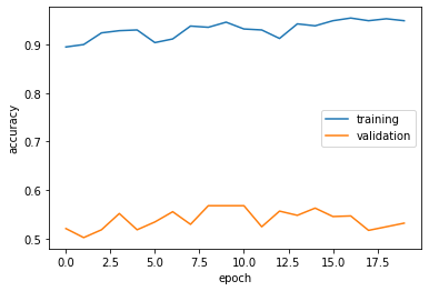
I tried experimenting with the number of Conv2D layers in my Model #1, since this is the meat and potato of Image Classification models. Eventually, the validation accuracy stabalizes around 53%, which slightly better than the baseline accuracy. Still, overfitting is observed. The training accuracy is significantly higher than validation accuracy.
Model with Data Augmentation
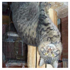
In this section, we will be employing Data Augmentation to improve our model. We will create a RandomFlip and RandomRotation layer to modify our existing dataset to improve the versatility of our model. Below are the effects of the augmentation layers.
#show an original image for comparison
image = None
for images, labels in train_dataset.take(1):
  for i in range(1):
    ax = plt.subplot(1, 1, i + 1)
    image = images[i]
    plt.imshow(image.numpy().astype("uint8"))
    plt.axis("off")

flip = layers.RandomFlip()

flipped = flip(image, training=True)
ax = plt.subplot(1, 1, 1)
plt.imshow(flipped.numpy().astype("uint8"))
plt.axis("off")
(-0.5, 159.5, 159.5, -0.5)
rotate = layers.RandomRotation(0.2)
rotated = rotate(image, training=True)
ax = plt.subplot(1, 1, 1)
plt.imshow(rotated.numpy().astype("uint8"))
plt.axis("off")
(-0.5, 159.5, 159.5, -0.5)

The above modified image could potentially help our model achieve better performace. We will apply these to our Model2.
model2 = keras.Sequential([
    #added data augmentation layer
    layers.RandomFlip(),
    layers.RandomRotation(0.2),

    #existing layers from before
    layers.Conv2D(32, (3, 3), activation='relu', input_shape=(160, 160, 3)),
    layers.MaxPooling2D((2, 2)),
    layers.Conv2D(32, (3, 3), activation='relu'),
    layers.MaxPooling2D((2, 2)),
    layers.Dropout(0.2),
    layers.Dense(64),
    layers.Flatten(),
    layers.Dense(2)
])

model2.compile(optimizer='adam',
              loss = tf.keras.losses.SparseCategoricalCrossentropy(from_logits=True),
              metrics = ['accuracy'])

history2 = model2.fit(train_dataset,
                   epochs=20, # how many rounds of training to do
                   validation_data = validation_dataset
)
Epoch 1/20
63/63 [==============================] - 66s 1s/step - loss: 213.6765 - accuracy: 0.5000 - val_loss: 1.5880 - val_accuracy: 0.5396
Epoch 2/20
63/63 [==============================] - 63s 1s/step - loss: 1.1807 - accuracy: 0.5505 - val_loss: 0.9861 - val_accuracy: 0.5520
Epoch 3/20
63/63 [==============================] - 64s 1s/step - loss: 0.8793 - accuracy: 0.5745 - val_loss: 0.8591 - val_accuracy: 0.5743
Epoch 4/20
63/63 [==============================] - 63s 1s/step - loss: 0.7875 - accuracy: 0.5560 - val_loss: 0.7763 - val_accuracy: 0.5656
Epoch 5/20
63/63 [==============================] - 63s 1s/step - loss: 0.7083 - accuracy: 0.5715 - val_loss: 0.7333 - val_accuracy: 0.5780
Epoch 6/20
63/63 [==============================] - 63s 1s/step - loss: 0.7146 - accuracy: 0.5795 - val_loss: 0.7183 - val_accuracy: 0.5322
Epoch 7/20
63/63 [==============================] - 64s 1s/step - loss: 0.6900 - accuracy: 0.5490 - val_loss: 0.6941 - val_accuracy: 0.5705
Epoch 8/20
63/63 [==============================] - 63s 1s/step - loss: 0.6921 - accuracy: 0.5615 - val_loss: 0.6931 - val_accuracy: 0.5606
Epoch 9/20
63/63 [==============================] - 64s 1s/step - loss: 0.6831 - accuracy: 0.5860 - val_loss: 0.6834 - val_accuracy: 0.5903
Epoch 10/20
63/63 [==============================] - 63s 1s/step - loss: 0.6865 - accuracy: 0.5910 - val_loss: 0.6971 - val_accuracy: 0.5767
Epoch 11/20
63/63 [==============================] - 63s 1s/step - loss: 0.6756 - accuracy: 0.5905 - val_loss: 0.6816 - val_accuracy: 0.5829
Epoch 12/20
63/63 [==============================] - 63s 1s/step - loss: 0.6778 - accuracy: 0.6020 - val_loss: 0.6793 - val_accuracy: 0.5879
Epoch 13/20
63/63 [==============================] - 63s 1s/step - loss: 0.6812 - accuracy: 0.5840 - val_loss: 0.6867 - val_accuracy: 0.5594
Epoch 14/20
63/63 [==============================] - 63s 1s/step - loss: 0.6697 - accuracy: 0.5945 - val_loss: 0.6731 - val_accuracy: 0.5953
Epoch 15/20
63/63 [==============================] - 64s 1s/step - loss: 0.6757 - accuracy: 0.6050 - val_loss: 0.6663 - val_accuracy: 0.5804
Epoch 16/20
63/63 [==============================] - 64s 1s/step - loss: 0.6619 - accuracy: 0.6040 - val_loss: 0.6541 - val_accuracy: 0.6151
Epoch 17/20
63/63 [==============================] - 63s 1s/step - loss: 0.6600 - accuracy: 0.6135 - val_loss: 0.6723 - val_accuracy: 0.6015
Epoch 18/20
63/63 [==============================] - 63s 1s/step - loss: 0.6526 - accuracy: 0.6305 - val_loss: 0.6916 - val_accuracy: 0.6077
Epoch 19/20
63/63 [==============================] - 63s 1s/step - loss: 0.6676 - accuracy: 0.6125 - val_loss: 0.6649 - val_accuracy: 0.6015
Epoch 20/20
63/63 [==============================] - 64s 1s/step - loss: 0.6492 - accuracy: 0.6395 - val_loss: 0.6893 - val_accuracy: 0.6114
#plot training and validation accuracy
plt.plot(history2.history["accuracy"], label = "training")
plt.plot(history2.history["val_accuracy"], label = "validation")
plt.gca().set(xlabel = "epoch", ylabel = "accuracy")
plt.legend()
<matplotlib.legend.Legend at 0x7fdf5becf3d0>
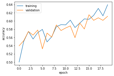
Model 2 with data augmentation stabalizes at around 60%, which is a huge improvement. Compared with Model 1, this is significantly better. Additionally, overfitting is less of an issue: testing and validation accuracies stay close throughout the 20 epochs.
Data Preprocessing
In this section, we will add data preprocessing to our model. By normalizing RGB values to -1 to 1, our model will hopefully train faster and perform better. Here’s the code for the preprocessing layer.
i = tf.keras.Input(shape=(160, 160, 3))
x = tf.keras.applications.mobilenet_v2.preprocess_input(i)
preprocessor = tf.keras.Model(inputs = [i], outputs = [x])
model3 = keras.Sequential([
    #preprocessing
    preprocessor,
    #added data augmentation layer
    layers.RandomFlip(),
    layers.RandomRotation(0.2),

    #existing layers from before
    layers.Conv2D(32, (3, 3), activation='relu', input_shape=(160, 160, 3)),
    layers.MaxPooling2D((2, 2)),
    layers.Conv2D(32, (3, 3), activation='relu'),
    layers.MaxPooling2D((2, 2)),
    layers.Conv2D(32, (3, 3), activation='relu'),
    layers.AveragePooling2D((2,2)),
    layers.Dropout(0.2),
    layers.Flatten(),
    layers.Dense(2)
    ])

model3.compile(optimizer='adam',
              loss = tf.keras.losses.SparseCategoricalCrossentropy(from_logits=True),
              metrics = ['accuracy'])

#train our model
history3 = model3.fit(train_dataset,
                   epochs=20, # how many rounds of training to do
                   validation_data = validation_dataset
)
Epoch 1/20
63/63 [==============================] - 72s 1s/step - loss: 0.6841 - accuracy: 0.5540 - val_loss: 0.6483 - val_accuracy: 0.5854
Epoch 2/20
63/63 [==============================] - 71s 1s/step - loss: 0.6427 - accuracy: 0.6140 - val_loss: 0.6348 - val_accuracy: 0.6349
Epoch 3/20
63/63 [==============================] - 72s 1s/step - loss: 0.6201 - accuracy: 0.6450 - val_loss: 0.5963 - val_accuracy: 0.6770
Epoch 4/20
63/63 [==============================] - 73s 1s/step - loss: 0.6010 - accuracy: 0.6695 - val_loss: 0.5860 - val_accuracy: 0.7116
Epoch 5/20
63/63 [==============================] - 71s 1s/step - loss: 0.5896 - accuracy: 0.6950 - val_loss: 0.5938 - val_accuracy: 0.6819
Epoch 6/20
63/63 [==============================] - 71s 1s/step - loss: 0.5788 - accuracy: 0.6945 - val_loss: 0.5494 - val_accuracy: 0.7030
Epoch 7/20
63/63 [==============================] - 72s 1s/step - loss: 0.5737 - accuracy: 0.6940 - val_loss: 0.5639 - val_accuracy: 0.6869
Epoch 8/20
63/63 [==============================] - 71s 1s/step - loss: 0.5597 - accuracy: 0.7150 - val_loss: 0.5399 - val_accuracy: 0.7290
Epoch 9/20
63/63 [==============================] - 72s 1s/step - loss: 0.5763 - accuracy: 0.6950 - val_loss: 0.5526 - val_accuracy: 0.7067
Epoch 10/20
63/63 [==============================] - 71s 1s/step - loss: 0.5557 - accuracy: 0.7135 - val_loss: 0.5613 - val_accuracy: 0.7005
Epoch 11/20
63/63 [==============================] - 72s 1s/step - loss: 0.5474 - accuracy: 0.7220 - val_loss: 0.5356 - val_accuracy: 0.7401
Epoch 12/20
63/63 [==============================] - 72s 1s/step - loss: 0.5459 - accuracy: 0.7175 - val_loss: 0.5390 - val_accuracy: 0.7339
Epoch 13/20
63/63 [==============================] - 74s 1s/step - loss: 0.5468 - accuracy: 0.7280 - val_loss: 0.5400 - val_accuracy: 0.7228
Epoch 14/20
63/63 [==============================] - 77s 1s/step - loss: 0.5328 - accuracy: 0.7395 - val_loss: 0.5254 - val_accuracy: 0.7314
Epoch 15/20
63/63 [==============================] - 73s 1s/step - loss: 0.5225 - accuracy: 0.7350 - val_loss: 0.5520 - val_accuracy: 0.7240
Epoch 16/20
63/63 [==============================] - 76s 1s/step - loss: 0.5273 - accuracy: 0.7345 - val_loss: 0.5469 - val_accuracy: 0.7079
Epoch 17/20
63/63 [==============================] - 81s 1s/step - loss: 0.5182 - accuracy: 0.7440 - val_loss: 0.5297 - val_accuracy: 0.7277
Epoch 18/20
63/63 [==============================] - 79s 1s/step - loss: 0.5247 - accuracy: 0.7340 - val_loss: 0.5704 - val_accuracy: 0.7030
Epoch 19/20
63/63 [==============================] - 84s 1s/step - loss: 0.5153 - accuracy: 0.7405 - val_loss: 0.5336 - val_accuracy: 0.7376
Epoch 20/20
63/63 [==============================] - 77s 1s/step - loss: 0.5259 - accuracy: 0.7450 - val_loss: 0.5138 - val_accuracy: 0.7364
#plot training and validation accuracy
plt.plot(history3.history["accuracy"], label = "training")
plt.plot(history3.history["val_accuracy"], label = "validation")
plt.gca().set(xlabel = "epoch", ylabel = "accuracy")
plt.legend()
<matplotlib.legend.Legend at 0x7fd06d7e8b90>
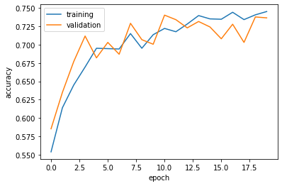
Model 3 stabalizes at over 70% accuracy. This is a huge improvement over Model 1 and Model 2. Overfitting is insignificant as training and testing accuracies are close.
Transfer Learning
In this section, we will transfer from an existing base model to our task: distinguishing from cats and dogs. We will be using MobileNetV2 as our base model.
#downloads the base model
IMG_SHAPE = IMG_SIZE + (3,)
base_model = tf.keras.applications.MobileNetV2(input_shape=IMG_SHAPE,
                                               include_top=False,
                                               weights='imagenet')
base_model.trainable = False

i = tf.keras.Input(shape=IMG_SHAPE)
x = base_model(i, training = False)
base_model_layer = tf.keras.Model(inputs = [i], outputs = [x])
Downloading data from https://storage.googleapis.com/tensorflow/keras-applications/mobilenet_v2/mobilenet_v2_weights_tf_dim_ordering_tf_kernels_1.0_160_no_top.h5
9412608/9406464 [==============================] - 0s 0us/step
9420800/9406464 [==============================] - 0s 0us/step
Time to train our model!
model4 = keras.Sequential([
    #preprocessing
    preprocessor,
    #added data augmentation layer
    layers.RandomFlip(),
    layers.RandomRotation(0.2),
    #base model
    base_model_layer,
    #added layers
    layers.GlobalMaxPooling2D(),
    layers.Dropout(0.2),
    layers.Flatten(),
    layers.Dense(2)
    ])

model4.compile(optimizer='adam',
              loss = tf.keras.losses.SparseCategoricalCrossentropy(from_logits=True),
              metrics = ['accuracy'])

model4.summary()
Model: "sequential_1"
_________________________________________________________________
 Layer (type)                Output Shape              Param #
=================================================================
 model_1 (Functional)        (None, 160, 160, 3)       0

 random_flip (RandomFlip)    (None, 160, 160, 3)       0

 random_rotation (RandomRota  (None, 160, 160, 3)      0
 tion)

 model (Functional)          (None, 5, 5, 1280)        2257984

 global_max_pooling2d (Globa  (None, 1280)             0
 lMaxPooling2D)

 dropout_1 (Dropout)         (None, 1280)              0

 flatten_1 (Flatten)         (None, 1280)              0

 dense_1 (Dense)             (None, 2)                 2562

=================================================================
Total params: 2,260,546
Trainable params: 2,562
Non-trainable params: 2,257,984
_________________________________________________________________
There are over 2,260,546 parameters to train! This is much larger that what we had by ourselves.
#trains our model
history4 = model4.fit(train_dataset,
                   epochs=20, # how many rounds of training to do
                   validation_data = validation_dataset
)
Epoch 1/20
63/63 [==============================] - 16s 114ms/step - loss: 0.8256 - accuracy: 0.7900 - val_loss: 0.1275 - val_accuracy: 0.9629
Epoch 2/20
63/63 [==============================] - 6s 88ms/step - loss: 0.4929 - accuracy: 0.8690 - val_loss: 0.1283 - val_accuracy: 0.9567
Epoch 3/20
63/63 [==============================] - 6s 89ms/step - loss: 0.4703 - accuracy: 0.8775 - val_loss: 0.1196 - val_accuracy: 0.9653
Epoch 4/20
63/63 [==============================] - 6s 88ms/step - loss: 0.4046 - accuracy: 0.8880 - val_loss: 0.1011 - val_accuracy: 0.9678
Epoch 5/20
63/63 [==============================] - 6s 88ms/step - loss: 0.4159 - accuracy: 0.8950 - val_loss: 0.0969 - val_accuracy: 0.9653
Epoch 6/20
63/63 [==============================] - 6s 89ms/step - loss: 0.3679 - accuracy: 0.8975 - val_loss: 0.1160 - val_accuracy: 0.9567
Epoch 7/20
63/63 [==============================] - 6s 88ms/step - loss: 0.3771 - accuracy: 0.8975 - val_loss: 0.1254 - val_accuracy: 0.9616
Epoch 8/20
63/63 [==============================] - 6s 88ms/step - loss: 0.3933 - accuracy: 0.8950 - val_loss: 0.0832 - val_accuracy: 0.9691
Epoch 9/20
63/63 [==============================] - 6s 90ms/step - loss: 0.3322 - accuracy: 0.9025 - val_loss: 0.1167 - val_accuracy: 0.9641
Epoch 10/20
63/63 [==============================] - 6s 88ms/step - loss: 0.3493 - accuracy: 0.9055 - val_loss: 0.0845 - val_accuracy: 0.9653
Epoch 11/20
63/63 [==============================] - 6s 89ms/step - loss: 0.3838 - accuracy: 0.8885 - val_loss: 0.1060 - val_accuracy: 0.9629
Epoch 12/20
63/63 [==============================] - 7s 99ms/step - loss: 0.3489 - accuracy: 0.8980 - val_loss: 0.0910 - val_accuracy: 0.9678
Epoch 13/20
63/63 [==============================] - 6s 90ms/step - loss: 0.2927 - accuracy: 0.9180 - val_loss: 0.0652 - val_accuracy: 0.9715
Epoch 14/20
63/63 [==============================] - 6s 88ms/step - loss: 0.3172 - accuracy: 0.9130 - val_loss: 0.0698 - val_accuracy: 0.9740
Epoch 15/20
63/63 [==============================] - 6s 89ms/step - loss: 0.2635 - accuracy: 0.9145 - val_loss: 0.0872 - val_accuracy: 0.9691
Epoch 16/20
63/63 [==============================] - 6s 89ms/step - loss: 0.3718 - accuracy: 0.9050 - val_loss: 0.0665 - val_accuracy: 0.9777
Epoch 17/20
63/63 [==============================] - 6s 89ms/step - loss: 0.2882 - accuracy: 0.9120 - val_loss: 0.1319 - val_accuracy: 0.9604
Epoch 18/20
63/63 [==============================] - 6s 89ms/step - loss: 0.2866 - accuracy: 0.9095 - val_loss: 0.0761 - val_accuracy: 0.9715
Epoch 19/20
63/63 [==============================] - 6s 88ms/step - loss: 0.2405 - accuracy: 0.9270 - val_loss: 0.0950 - val_accuracy: 0.9715
Epoch 20/20
63/63 [==============================] - 6s 89ms/step - loss: 0.2840 - accuracy: 0.9080 - val_loss: 0.0782 - val_accuracy: 0.9740
#plot training and validation accuracy
plt.plot(history4.history["accuracy"], label = "training")
plt.plot(history4.history["val_accuracy"], label = "validation")
plt.gca().set(xlabel = "epoch", ylabel = "accuracy")
plt.legend()
<matplotlib.legend.Legend at 0x7fdbc2e22c90>
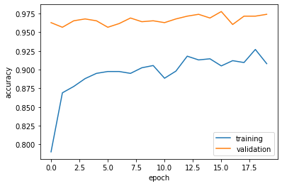
Our transfer learning model is able to achieve over 95% accuracy. This is significantly better than the previous models. Overfitting is observed, but better than previous models.
Test Data
We will now apply Model 4, our best performer so far, on your test model.
#saves the test results
score = model4.evaluate(test_dataset)
score
6/6 [==============================] - 1s 66ms/step - loss: 0.0714 - accuracy: 0.9792


[0.07144574075937271, 0.9791666865348816]
We are able to achieve 97.92% accuracy, which is impressive!