Detecting Fake News with Natural Language Processing

In this blog post, we will train some natural language processing models to classify fake news.

Data Acquisition

import pandas as pd
import tensorflow as tf
from matplotlib import pyplot as plt

train_url = "https://github.com/PhilChodrow/PIC16b/blob/master/datasets/fake_news_train.csv?raw=true"
df = pd.read_csv(train_url)

The dataframe consists of many news articles. The title and text are separated into different columns. Articles containing fake news information are labelled with 1 in the last column. Let’s take a look.

df.head()

	Unnamed: 0	title	text	fake
0	17366	Merkel: Strong result for Austria's FPO 'big c...	German Chancellor Angela Merkel said on Monday...	0
1	5634	Trump says Pence will lead voter fraud panel	WEST PALM BEACH, Fla.President Donald Trump sa...	0
2	17487	JUST IN: SUSPECTED LEAKER and “Close Confidant...	On December 5, 2017, Circa s Sara Carter warne...	1
3	12217	Thyssenkrupp has offered help to Argentina ove...	Germany s Thyssenkrupp, has offered assistance...	0
4	5535	Trump say appeals court decision on travel ban...	President Donald Trump on Thursday called the ...	0

Dataset Construction

Make a dataset

We will first have to remove all stop words, such as “and”, “at”, etc. from our dataframe. Then, we will transform our dataframe into a tf.dataset object.

#import a list of stop words
import nltk 
from nltk.corpus import stopwords
from sklearn.preprocessing import LabelEncoder
nltk.download('stopwords')
stop = stopwords.words('english')

def make_dataset(df):
  """
  A function that takes in a pd dataframe that contains news articles, removes stop words, and returns a tf.data.dataset object
  """
  #cleans up the labels
  le = LabelEncoder()
  df["fake"] = le.fit_transform(df["fake"])
  num_title = len(df["fake"].unique())

  #remove stop words from title and text
  df['title'] = df['title'].apply(lambda x: ' '.join([word for word in x.split() if word not in (stop)]))
  df['text'] = df['text'].apply(lambda x: ' '.join([word for word in x.split() if word not in (stop)]))

  #converts into a tf dataset
  data = tf.data.Dataset.from_tensor_slices((
    # dictionary for input data/features
      { "title": df[["title"]],
     "text": df[["text"]]
    },
    # dictionary for output data/labels
    { "fake": df["fake"]
        
    }))
  return data

[nltk_data] Downloading package stopwords to /root/nltk_data...
[nltk_data]   Unzipping corpora/stopwords.zip.

data = make_dataset(df)

data.take(1)

<TakeDataset element_spec=({'title': TensorSpec(shape=(1,), dtype=tf.string, name=None), 'text': TensorSpec(shape=(1,), dtype=tf.string, name=None)}, {'fake': TensorSpec(shape=(), dtype=tf.int64, name=None)})>

Validation Data

data = data.shuffle(buffer_size = len(data))

train_size = int(0.8*len(data)) 
val_size = int(0.2*len(data))

train = data.take(train_size) # data[:train_size]
val = data.skip(train_size).take(val_size) # data[train_size : train_size + val_size]

train = data.take(train_size).batch(20)
val = data.skip(train_size).take(val_size).batch(20)

Base Rate

Let’s examine the base accuracy rate of our model, i.e. what percentages of articles are fake. To do this, we will implement a fake news iterator first.

f_count = len(df[df["fake"] == 1])
r_count = len(df[df["fake"] == 0])

(len(df), r_count, f_count)

(22449, 10709, 11740)

There are 10709 fake news articles and 11740 legitimate news articles out of a total of 22449 articles. The fake news rate is 52.3%.

Text Vectorization

We will be using the TextVectorization API from the keras library to process our data. We will also convert all letters to lower case and get rid of all punctuations

from tensorflow.keras.layers.experimental.preprocessing import TextVectorization
import re
import string

#preparing a text vectorization layer for tf model
size_vocabulary = 2000

def standardization(input_data):
    lowercase = tf.strings.lower(input_data)
    no_punctuation = tf.strings.regex_replace(lowercase,
                                  '[%s]' % re.escape(string.punctuation),'')
    return no_punctuation 

title_vectorize_layer = TextVectorization(
    standardize=standardization,
    max_tokens=size_vocabulary, # only consider this many words
    output_mode='int',
    output_sequence_length=500) 

title_vectorize_layer.adapt(train.map(lambda x, y: x["title"]))

Models

We will be creating three models: one with just the title as input, one with just the text, and one with both.

Model 1

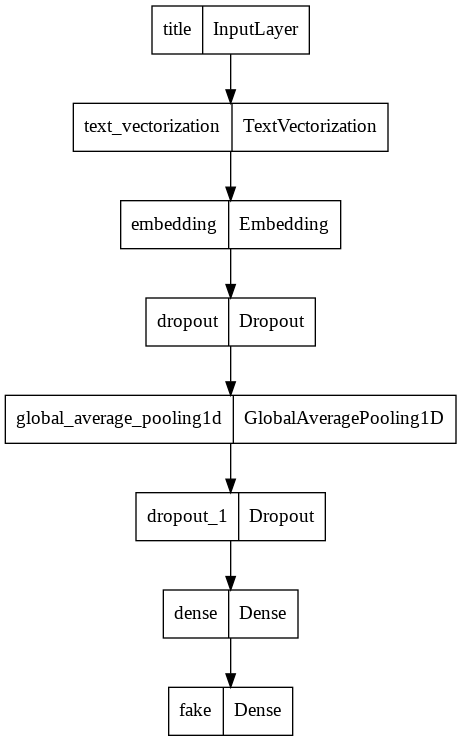
Model 1 will be trained using only the title. We will be using the Functional API from keras.

from tensorflow.keras import layers
from tensorflow import keras

#standardizes the labels
num_fake = len(df["fake"].unique())

#specifies the input layer
title_input = keras.Input(
    shape=(1,),
    name = "title", # same name as the dictionary key in the dataset
    dtype = "string"
)

#the feature layers
title_features = title_vectorize_layer(title_input)
title_features = layers.Embedding(size_vocabulary, output_dim = 3, name="embedding")(title_features)
title_features = layers.Dropout(0.2)(title_features)
title_features = layers.GlobalAveragePooling1D()(title_features)
title_features = layers.Dropout(0.2)(title_features)
title_features = layers.Dense(32, activation='relu')(title_features)

output = layers.Dense(num_fake, name="fake")(title_features) 

model1 = keras.Model(
    inputs = title_input,
    outputs = output
)

keras.utils.plot_model(model1)

png

from tensorflow.keras import losses

model1.compile(optimizer="adam",
              loss = losses.SparseCategoricalCrossentropy(from_logits=True),
              metrics=["accuracy"])

history = model1.fit(train, 
                    validation_data=val,
                    epochs = 30,
                    verbose = False)

/usr/local/lib/python3.7/dist-packages/keras/engine/functional.py:559: UserWarning:

Input dict contained keys ['text'] which did not match any model input. They will be ignored by the model.

Now let’s see how well our first model has performed.

from matplotlib import pyplot as plt
plt.plot(history.history["accuracy"], label = "training")
plt.plot(history.history["val_accuracy"], label = "validation")
plt.gca().set(xlabel = "epoch", ylabel = "accuracy")
plt.legend()

<matplotlib.legend.Legend at 0x7f22fdd7a650>

png

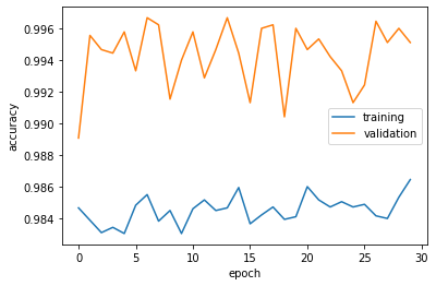
Validation accuracy stabalizes at around 98%, which is extremely impressive compared with a base rate of 52.3%. Overfitting is not a significant concern.

Model 2

For our second model, we will keep things mostly the same, except that we will be using only the article text for training.

#using the text column as input
text_input = keras.Input(
    shape=(1,),
    name = "text", # same name as the dictionary key in the dataset
    dtype = "string"
)

#the rest of model 2 is exactly the same as model 1
text_features = title_vectorize_layer(text_input)
text_features = layers.Embedding(size_vocabulary, output_dim = 3, name="embedding")(text_features)
text_features = layers.Dropout(0.2)(text_features)
text_features = layers.GlobalAveragePooling1D()(text_features)
text_features = layers.Dropout(0.2)(text_features)
text_features = layers.Dense(32, activation='relu')(text_features)

output = layers.Dense(num_fake, name="fake")(text_features) 

model2 = keras.Model(
    inputs = text_input,
    outputs = output
)

model2.compile(optimizer="adam",
              loss = losses.SparseCategoricalCrossentropy(from_logits=True),
              metrics=["accuracy"])

history = model2.fit(train, 
                    validation_data=val,
                    epochs = 30,
                    verbose = False)

/usr/local/lib/python3.7/dist-packages/keras/engine/functional.py:559: UserWarning:

Input dict contained keys ['title'] which did not match any model input. They will be ignored by the model.

plt.plot(history.history["accuracy"], label = "training")
plt.plot(history.history["val_accuracy"], label = "validation")
plt.gca().set(xlabel = "epoch", ylabel = "accuracy")
plt.legend()

<matplotlib.legend.Legend at 0x7f242679f790>

png

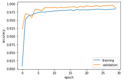
Model 2 has performed just as well, but takes slightly longer to train.

Model 3

For the third model, we will fully take advantage of the Keras Functional API by using both article title and text as our input layer.

#using the title column as input
title_input = keras.Input(
    shape=(1,),
    name = "title", # same name as the dictionary key in the dataset
    dtype = "string"
)

#using the text column as input
text_input = keras.Input(
    shape=(1,),
    name = "text", # same name as the dictionary key in the dataset
    dtype = "string"
)

#layers handling the title input
title_features = title_vectorize_layer(title_input)
title_features = layers.Embedding(size_vocabulary, output_dim = 3, name="embedding1")(title_features)
title_features = layers.Dropout(0.2)(title_features)
title_features = layers.GlobalAveragePooling1D()(title_features)
title_features = layers.Dropout(0.2)(title_features)
title_features = layers.Dense(32, activation='relu')(title_features)

#layers handling the text input
text_features = title_vectorize_layer(text_input)
text_features = layers.Embedding(size_vocabulary, output_dim = 3, name="embedding2")(text_features)
text_features = layers.Dropout(0.2)(text_features)
text_features = layers.GlobalAveragePooling1D()(text_features)
text_features = layers.Dropout(0.2)(text_features)
text_features = layers.Dense(32, activation='relu')(text_features)

#concatenates the two input branches into one main layer                                                    
main = layers.concatenate([title_features, text_features], axis = 1)
main = layers.Dense(32, activation='relu')(main)

#output is the same as before
output = layers.Dense(num_fake, name="fake")(main) 

#makes our third model
model3 = keras.Model(
    inputs = [title_input, text_input],
    outputs = output
)

keras.utils.plot_model(model3)

png

As shown above, our third model starts from having two branches, one on text the other on title, before being concatenated into a final output. Let’s see how it performs.

model3.compile(optimizer="adam",
              loss = losses.SparseCategoricalCrossentropy(from_logits=True),
              metrics=["accuracy"])
history = model3.fit(train, 
                    validation_data=val,
                    epochs = 30,
                    verbose = False)

plt.plot(history.history["accuracy"], label = "training")
plt.plot(history.history["val_accuracy"], label = "validation")
plt.gca().set(xlabel = "epoch", ylabel = "accuracy")
plt.legend()

<matplotlib.legend.Legend at 0x7f24266f3890>

png

Our third model has performed the best so far, consistently scoring close to 100% accuracy. Overfitting is not observed. Ideally, the fake news detection algorithm would be trained on both the title and the text.

Evaluating our Best Model

We will be using a fresh dataset to evaluate our best model, model 3. First let’s import this dataframe and make it a dataset.

#data import and conversion into dataset
test_url = "https://github.com/PhilChodrow/PIC16b/blob/master/datasets/fake_news_test.csv?raw=true"
df_test = pd.read_csv(test_url)
data = make_dataset(df_test)

#Let's look at the base rate for the testing dataset
f_count = len(df_test[df_test["fake"] == 1])
r_count = len(df_test[df_test["fake"] == 0])

(len(df), r_count, f_count)

(22449, 10708, 11741)

The base rate is right around 50% still.

data = data.shuffle(buffer_size = len(data))
test = data.batch(20)

model3.evaluate(test)

1123/1123 [==============================] - 5s 4ms/step - loss: 0.0203 - accuracy: 0.9938

[0.020348409190773964, 0.9938082098960876]

Our best model has scored a whopping 99.38% accuracy on the unseen testing dataset, against a base rate of just over 50%. In the real world, our model has great potentials telling apart fake news.

Embedding Visualization

Let’s look at how our text embedding layers work!

weights2 = model3.get_layer('embedding2').get_weights()[0] # get the weights from the embedding layer
vocab = title_vectorize_layer.get_vocabulary()                # get the vocabulary from our data prep for later

from sklearn.decomposition import PCA
pca = PCA(n_components=2)
weights2 = pca.fit_transform(weights2)

embedding_df = pd.DataFrame({
    'word' : vocab, 
    'x0'   : weights2[:,0],
    'x1'   : weights2[:,1]
})

import plotly.express as px 
from plotly.io import write_html

fig = px.scatter(embedding_df, 
                 x = "x0", 
                 y = "x1", 
                 size = [2]*len(embedding_df),
                # size_max = 2,
                 hover_name = "word")

fig.show()
write_html(fig, "embedding.html")

It appears that words like “lawsuit,” “news,” “attorney,” and “agents” are fairly neutral in our embedding layer, as they appear clustered around the origin in the plot above. These words appear universally in fabricated and legitimate news, thus cannot provide much insight on the nature of the article.

Towards the extremes of the plot we see words like “trump” and “gop.” These words are often controversial and likely included in fake news articles to grab attention. Creators of fake news are after internet traffic and will employ the most controversial rhetoric.

Written on May 15, 2022